CSC350 IntelligSys: Evolution of Computer Vision Presentation

Evolution of Computer Vision

A Review of Traditional and Deep Learning Approaches

Author

Kinshu Gupta

Origins

It all started with CNNs
Foundation of recent advances in computer vision
Architectures based on this model have been the most successful in the field

Origins: Cat Neural Networks (CNNs)

I am obviously talking about Cat Neural Networks (this is a satirical point, not an inaccuracy in my presentation)

Receptive fields of single neurones in the cat’s striate cortex

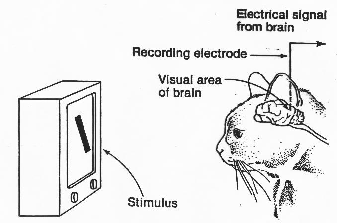
I dabble in neuroscience

Psychology: Bottom-Up Processing

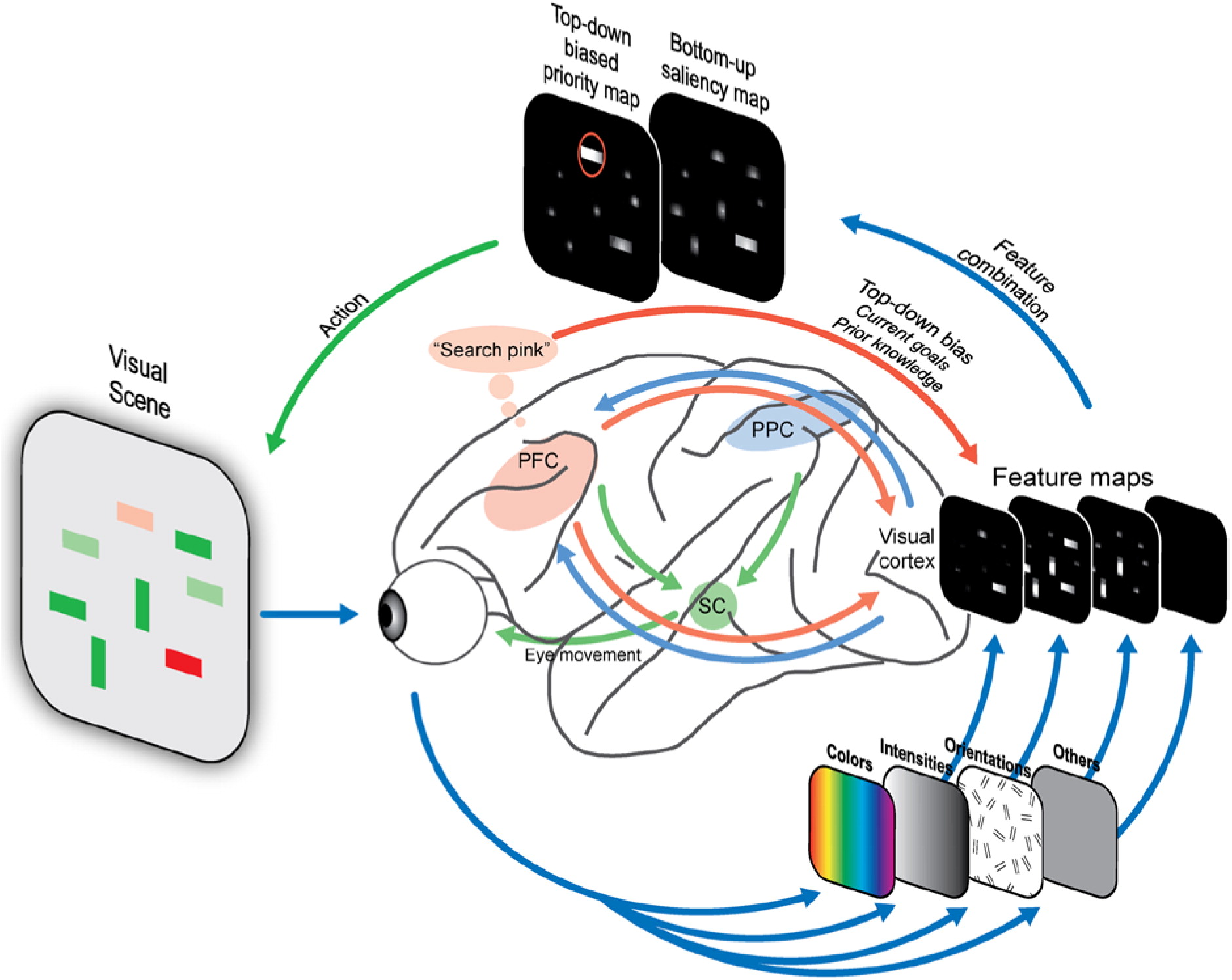
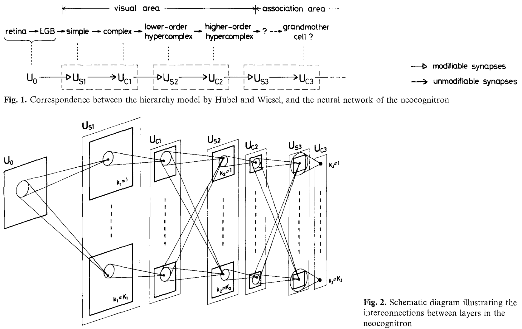
hierarchy structure : LGB (lateral geniculate body) -> simple cells -> complex cells -> lower order hypercomplex cells -> higher order hypercomplex cells

Neocognitron

neural networks to process images existed before, innovation is making it “deep” with convolutional layers basically first deep learning for CV

What are images?

import numpy as np
import matplotlib.pyplot as plt
import os
from pathlib import Path
from scipy.signal import convolve2d

img = plt.imread('images/bean.png')
gray_img = np.mean(img, axis=2)

fig, ax = plt.subplots(1, 2)
ax[0].imshow(img)
ax[1].imshow(gray_img, cmap='gray')
plt.show()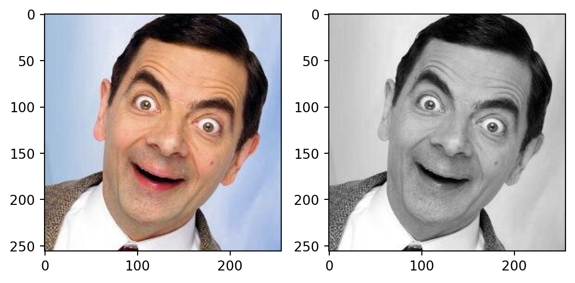

Images as Functions

def gaussian_kernel(size, sigma=1):
    size = int(size) // 2
    x, y = np.mgrid[-size:size+1, -size:size+1]
    normal = 1 / (2.0 * np.pi * sigma**2)
    g =  np.exp(-((x**2 + y**2) / (2.0*sigma**2))) * normal
    return g

kernel = gaussian_kernel(5, sigma=1)

blurred = convolve2d(gray_img, kernel, mode='same')

X = np.arange(gray_img.shape[0])
Y = np.arange(gray_img.shape[1])
X, Y = np.meshgrid(X, Y)

fig, ax = plt.subplots(subplot_kw={"projection": "3d"}); fig.set_size_inches(8, 7)
surf = ax.plot_surface(X, Y, 1 - np.flipud(blurred), cmap='summer')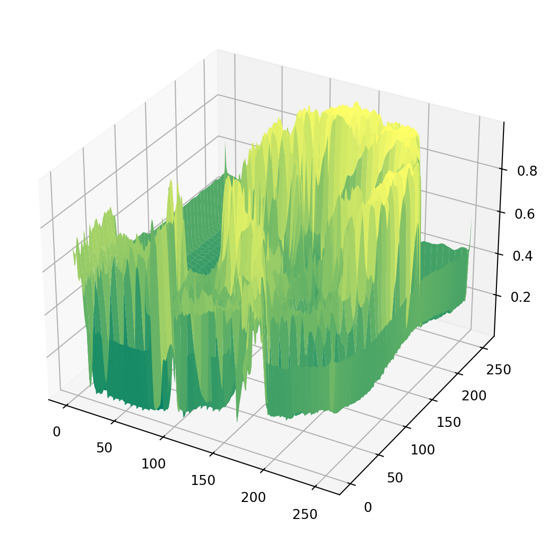

\(f\left(x,\ y\right)=\)

How to detect edges?

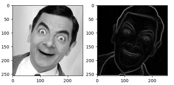
Gradients

Steep cliffs where intensity changes rapidly
Use some calculus
\(\nabla f = \begin{bmatrix} \frac{\partial f}{\partial x} \\ \frac{\partial f}{\partial y} \end{bmatrix}\)

fig, ax = plt.subplots(1, 3); fig.set_figwidth(12)

bounded = gray_img.copy()
bounded[49:150, 49] = 0
bounded[49:150, 150] = 0
bounded[49, 49:150] = 0
bounded[150, 49:150] = 0

bounded_2 = gray_img.copy()
bounded_2[80:115, 85] = 0
bounded_2[80:115, 120] = 0
bounded_2[80, 85:120] = 0
bounded_2[115, 85:120] = 0

ax[0].imshow(bounded, cmap='gray')
ax[1].imshow(bounded_2[49:150, 49:150], cmap='gray')
ax[2].imshow(gray_img[80:115, 85:120], cmap='gray')
plt.show()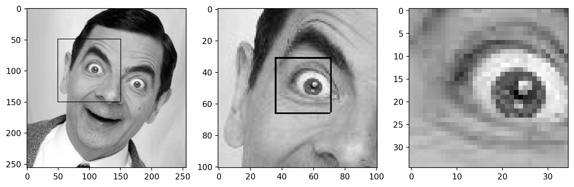

Convolution

Sobel

sobel_x = np.array([[-1, 0, 1],
                    [-2, 0, 2],
                    [-1, 0, 1]])
# sobel operator for y-direction
sobel_y = np.array([[1, 2, 1],
                    [0, 0, 0],
                    [-1, -2, -1]])

Sobel Linear Filter

convolved_x = convolve2d(blurred, sobel_x, mode='same')
convolved_y = convolve2d(blurred, sobel_y, mode='same')
combined_edges = np.sqrt(convolved_x**2 + convolved_y**2)

fig, ax = plt.subplots(1, 3)
fig.set_figwidth(12)
ax[0].imshow(convolved_x, cmap='gray')
ax[0].set_title('Horizontal Edges', y=-0.25)
ax[1].imshow(convolved_y, cmap='gray')
ax[1].set_title('Vertical Edges', y=-0.25)
ax[2].imshow(combined_edges, cmap='gray')
ax[2].set_title('Norm Edges', y=-0.25)
plt.show()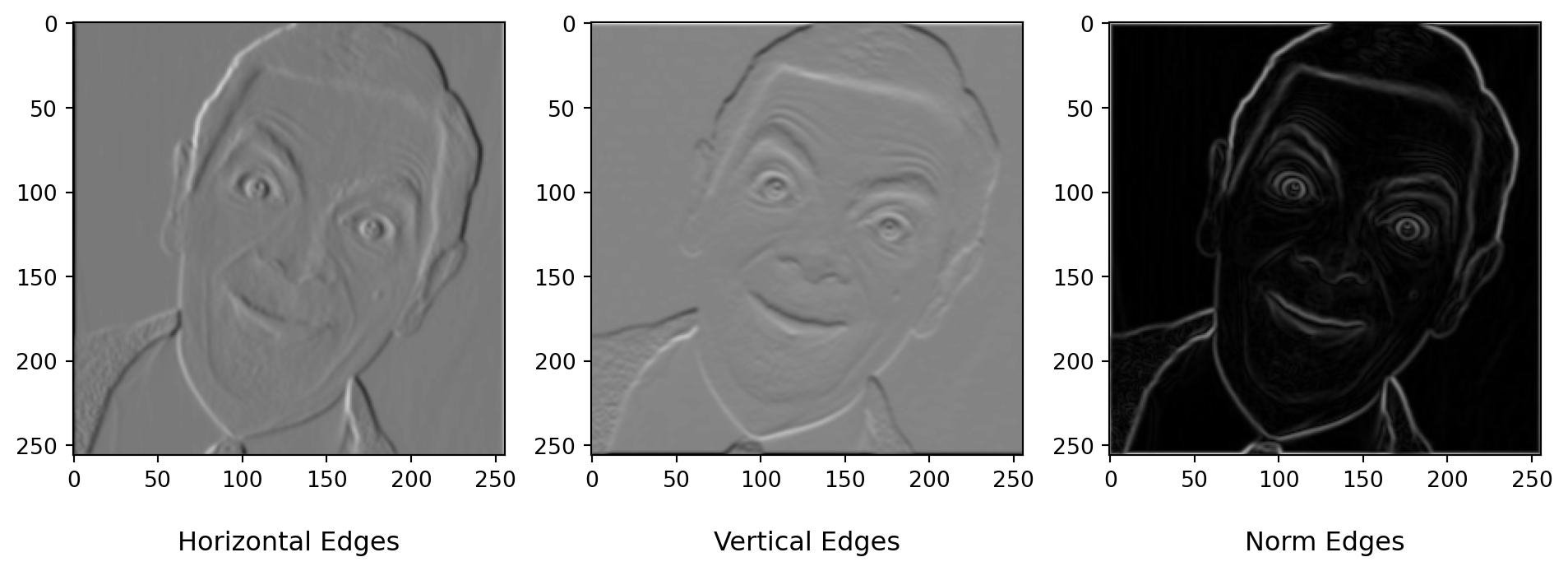

Other Filters

mean_kernel = np.ones((3, 3))

sharpen_kernel = np.array([[0, -1, 0],
                           [-1, 5, -1],
                           [0, -1, 0]])

impulse_kernel = np.array([[0, 0, 0],
                           [0, 1, 0],
                           [0, 0, 0]])

mean_blurred = convolve2d(gray_img, mean_kernel, mode='same')

sharpened = convolve2d(gray_img, sharpen_kernel, mode='same')
sharpened = np.clip(sharpened, 0, 1)

impulse = convolve2d(gray_img, impulse_kernel, mode='same')

fig, ax = plt.subplots(2, 3)
fig.set_size_inches(12, 7.5)
ax[0][0].imshow(mean_kernel, cmap='gray')
ax[0][0].set_title('Mean Kernel', y=-0.2)
ax[0][1].imshow(sharpen_kernel, cmap='gray')
ax[0][1].set_title('Sharpen Kernel', y=-0.2)
ax[0][2].imshow(impulse_kernel, cmap='gray')
ax[0][2].set_title('Impulse Kernel', y=-0.2)

kernels = [mean_kernel, sharpen_kernel, impulse_kernel]

for i in range(3):
  for r in range(3):
    for c in range(3):
      ax[0][i].text(c, r, kernels[i][r, c], ha="center", va="center", color="g", fontsize="large")

ax[1][0].imshow(mean_blurred / 9, cmap='gray')
ax[1][0].set_title('Mean Blur', y=-0.2)
ax[1][1].imshow(sharpened, cmap='gray')
ax[1][1].set_title('Sharpen', y=-0.2)
ax[1][2].imshow(impulse, cmap='gray')
ax[1][2].set_title('Impulse', y=-0.2)
plt.show()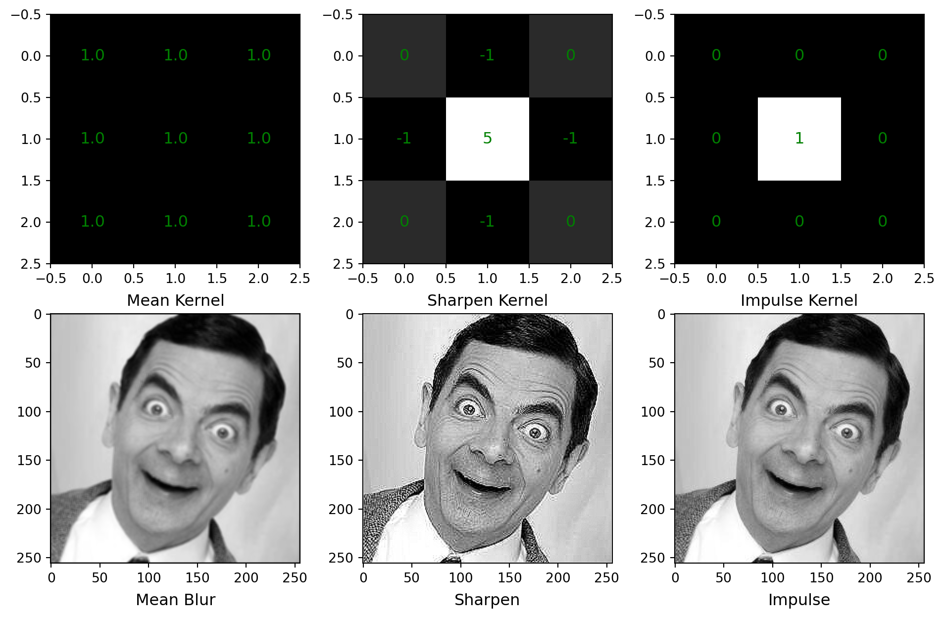

Traditional Computer Vision

Preprocessing: Denoising, Edge Detection, Subsampling
Segmentation: Thresholding, Active Contours
Feature Extraction: Scale Invariant Feature Transform (SIFT), Speeded Up Robust Features (SURF)

Dimension Reduction: PCA
Classification: Support Vector Machines (SVM), Random Forests, Boosting, Bagging, K-Nearest Neighbors (KNN)

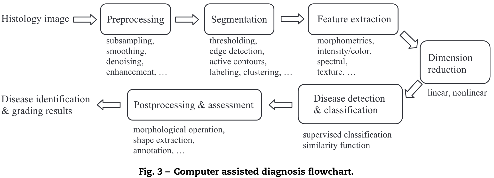
Domain: Computer Aided Diagnosis

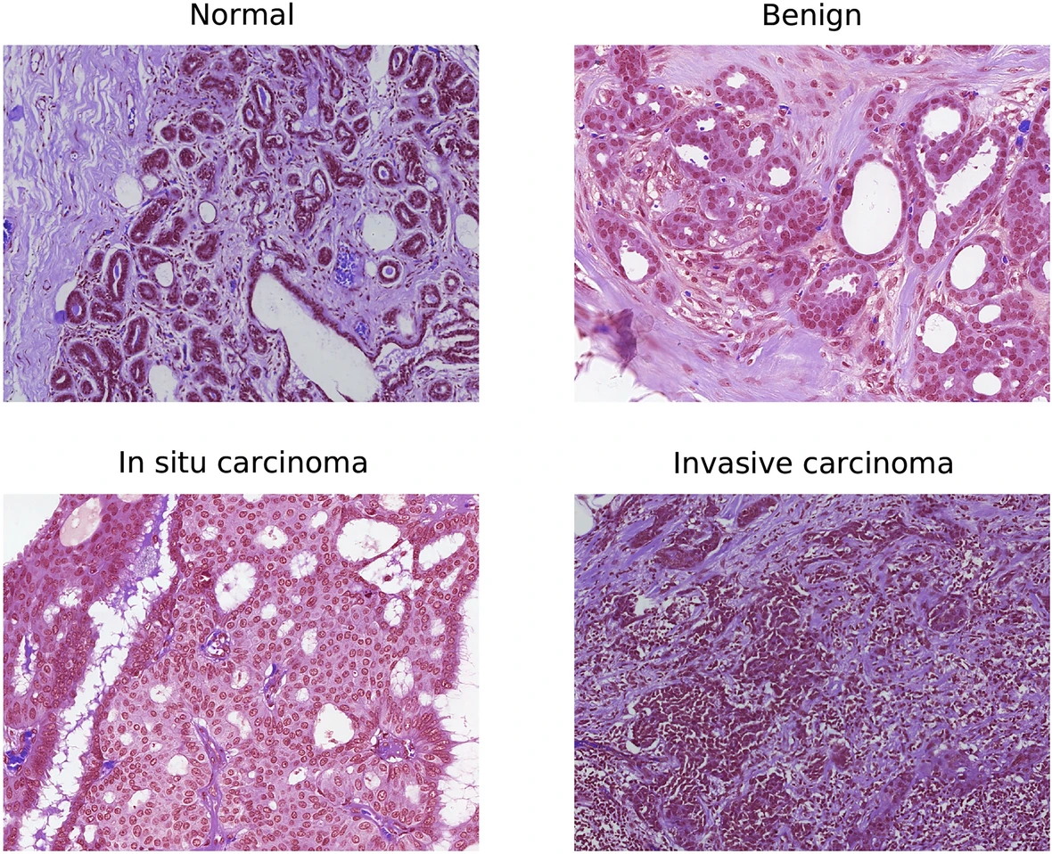
Diagnosis Pipeline

LeNet-5

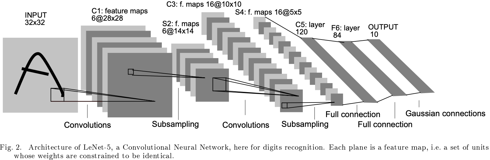
First Convolutional Neural Network as we know it today

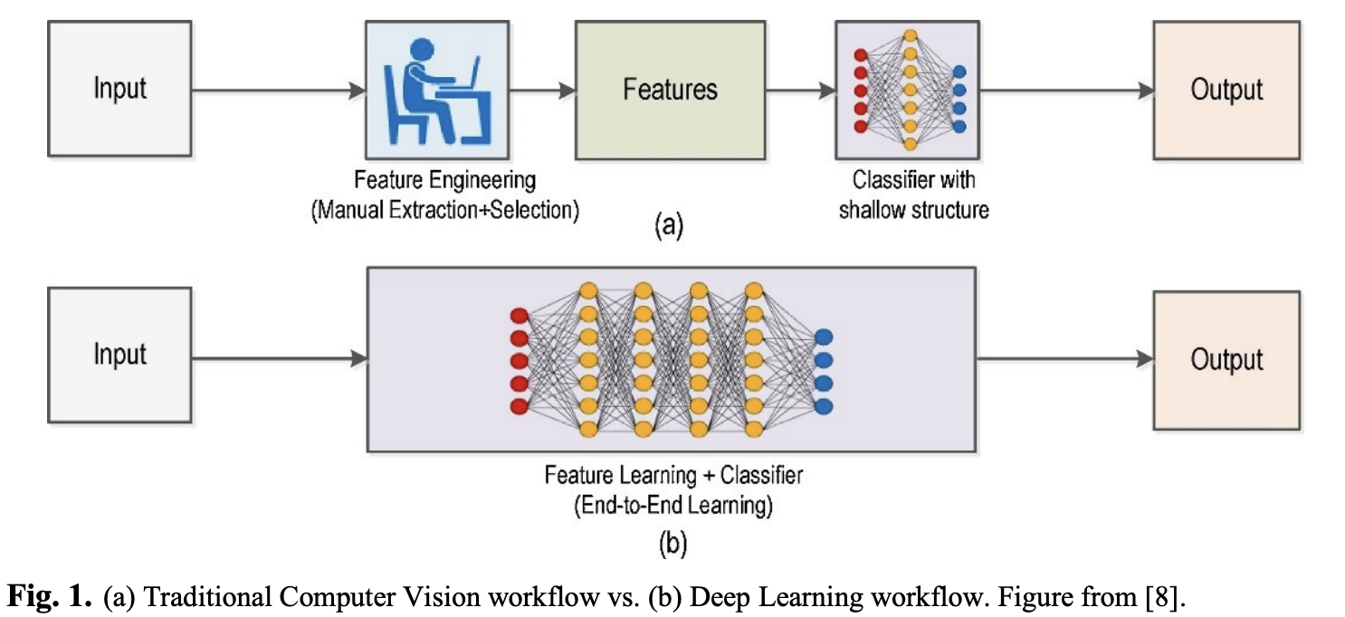
Comparison

One Small Step

Limitations of the Past

Lack of large structured datasets
Lack of computational power

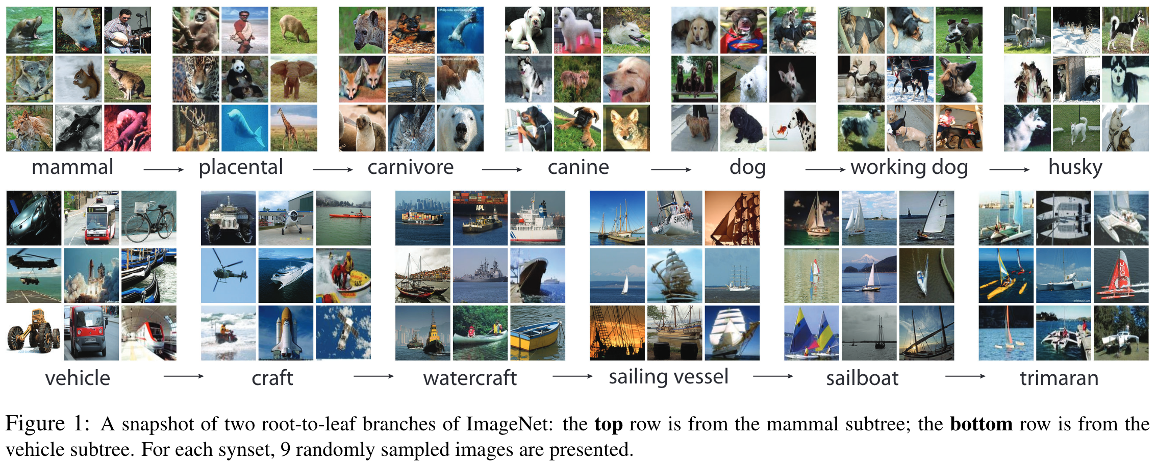
ImageNet: A Large-Scale Hierarchical Image Database

3.2 million images at time of publication
PASCAL VOC
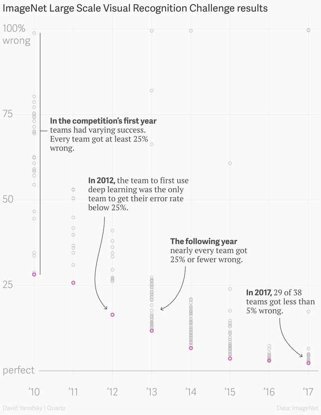
ImageNet Large Scale Visual Recognition Challenge (ILSVRC)

Fei-Fei Li

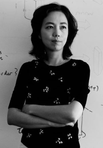
ImageNet: Snapshot

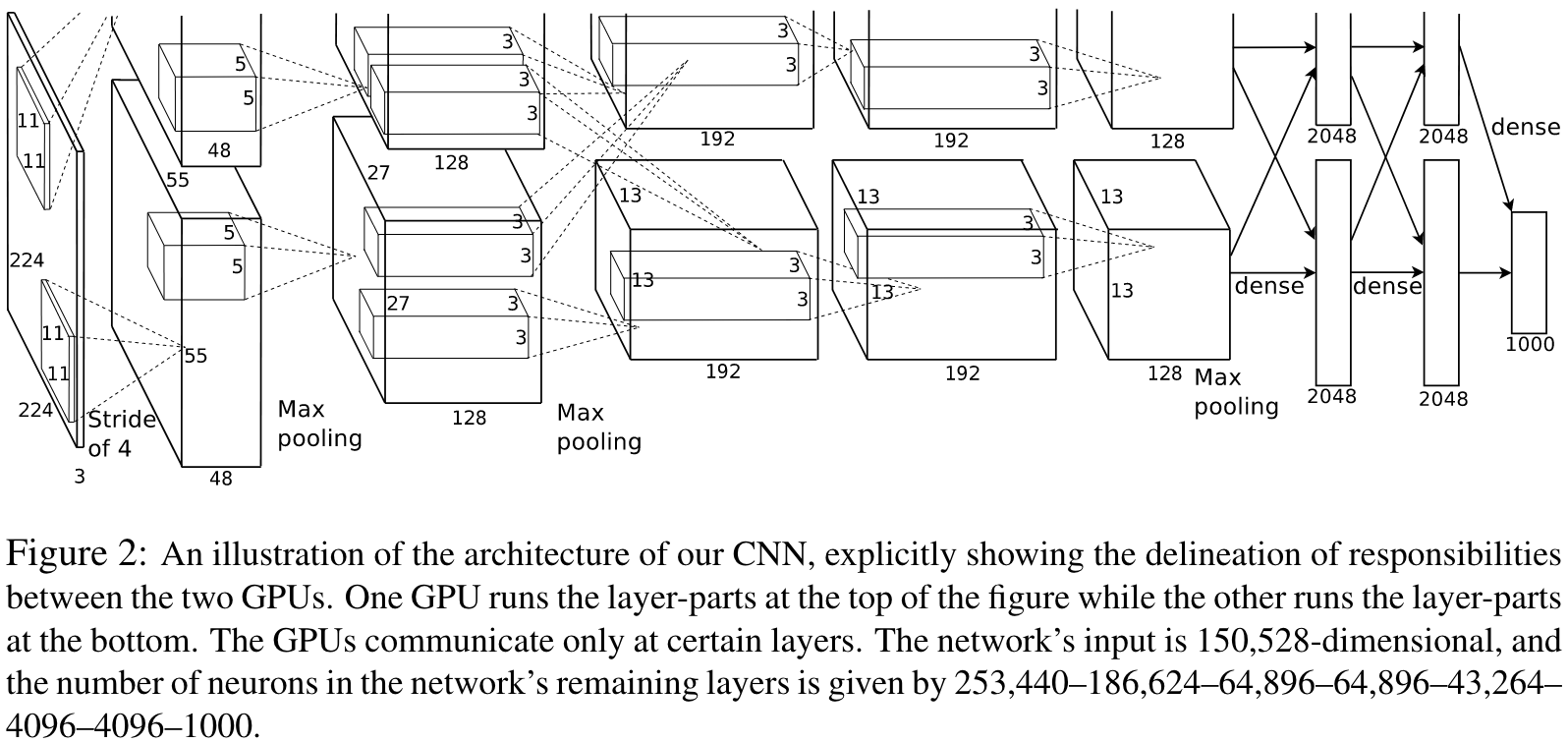
Breakthrough: AlexNet

Imagenet has 15 million images at this point
1.2 million images used to train
60 million parameters; 5 convolutional layers
Cross-GPU parallelization (2x GTX 580)
Non-saturating neurons (ReLU instead of tanh)
Overfitting: Dropout, Data Augmentation (cropping, flipping, color shifting) (training size effectively x2048)

ImageNet Classification with Deep Convolutional Neural Networks: Architecture

Review

Traditional Techniques

Tedious and time consuming
Infeasible for complex images
FAST

Deep Learning

“Easy”
LARGE datasets
Expensive compute

Hybrid / Mixed Approaches
Rare cancer detection is hard

References

[1] Jia Deng, Wei Dong, Richard Socher, Li-Jia Li, Kai Li, and Li Fei-Fei. 2009. ImageNet: A large-scale hierarchical image database. In 2009 IEEE Conference on Computer Vision and Pattern Recognition, June 2009. 248–255. . https://doi.org/10.1109/CVPR.2009.5206848

[2] Kunihiko Fukushima. 1988. Neocognitron: A hierarchical neural network capable of visual pattern recognition. Neural Networks 1, 2 (January 1988), 119–130. https://doi.org/10.1016/0893-6080(88)90014-7

[3] Zabit Hameed, Begonya Garcia-Zapirain, José Javier Aguirre, and Mario Arturo Isaza-Ruget. 2022. Multiclass classification of breast cancer histopathology images using multilevel features of deep convolutional neural network. Sci Rep 12, 1 (September 2022), 15600. https://doi.org/10.1038/s41598-022-19278-2

[4] Lei He, L. Rodney Long, Sameer Antani, and George R. Thoma. 2012. Histology image analysis for carcinoma detection and grading. Computer Methods and Programs in Biomedicine 107, 3 (September 2012), 538–556. https://doi.org/10.1016/j.cmpb.2011.12.007

[5] D. H. Hubel and T. N. Wiesel. 1959. Receptive fields of single neurones in the cat’s striate cortex. J Physiol 148, 3 (October 1959), 574–591.

[6] Fumi Katsuki and Christos Constantinidis. 2014. Bottom-Up and Top-Down Attention: Different Processes and Overlapping Neural Systems. Neuroscientist 20, 5 (October 2014), 509–521. https://doi.org/10.1177/1073858413514136

[7] Alex Krizhevsky, Ilya Sutskever, and Geoffrey E Hinton. 2012. ImageNet Classification with Deep Convolutional Neural Networks. In Advances in Neural Information Processing Systems, 2012. Curran Associates, Inc. . Retrieved December 1, 2023 from https://papers.nips.cc/paper_files/paper/2012/hash/c399862d3b9d6b76c8436e924a68c45b-Abstract.html

[8] Brajesh Kumar. 2021. Convolutional Neural Networks: A Brief History of their Evolution. AppyHigh Blog. Retrieved December 1, 2023 from https://medium.com/appyhigh-technology-blog/convolutional-neural-networks-a-brief-history-of-their-evolution-ee3405568597

[9] Yann LeCun, Leon Bottou, Yoshua Bengio, and Patrick Ha. 1998. Gradient-Based Learning Applied to Document Recognition. (1998).

[10] Niall O’ Mahony, Sean Campbell, Anderson Carvalho, Suman Harapanahalli, Gustavo Velasco-Hernandez, Lenka Krpalkova, Daniel Riordan, and Joseph Walsh. 2020. Deep Learning vs. Traditional Computer Vision. https://doi.org/10.1007/978-3-030-17795-9

[11] Irhum Shafkat. 2018. Intuitively Understanding Convolutions for Deep Learning. Medium. Retrieved December 3, 2023 from https://towardsdatascience.com/intuitively-understanding-convolutions-for-deep-learning-1f6f42faee1

[12] Richard Szeliski. 2022. Computer Vision: Algorithms and Applications. Springer International Publishing, Cham. https://doi.org/10.1007/978-3-030-34372-9

[13] Xiongwei Wu, Doyen Sahoo, and Steven C. H. Hoi. 2020. Recent advances in deep learning for object detection. Neurocomputing 396, (July 2020), 39–64. https://doi.org/10.1016/j.neucom.2020.01.085

[14] 2017. The data that transformed AI research—and possibly the world. Quartz. Retrieved December 1, 2023 from https://qz.com/1034972/the-data-that-changed-the-direction-of-ai-research-and-possibly-the-world

[15] A Brief History of Computer Vision (and Convolutional Neural Networks) | HackerNoon. Retrieved December 1, 2023 from https://hackernoon.com/a-brief-history-of-computer-vision-and-convolutional-neural-networks-8fe8aacc79f3

[16] CS5670: Introduction to Computer Vision, Spring 2023 – Cornell Tech. Retrieved December 2, 2023 from https://www.cs.cornell.edu/courses/cs5670/2023sp/

Other Formats

Origins

Origins: Cat Neural Networks (CNNs)

I dabble in neuroscience

Neocognitron

What are images?

Images as Functions

How to detect edges?

Gradients

Convolution

Convolution

Sobel

Sobel Linear Filter

Other Filters

Traditional Computer Vision

Domain: Computer Aided Diagnosis

Diagnosis Pipeline

LeNet-5

Comparison

One Small Step

ImageNet: A Large-Scale Hierarchical Image Database

ImageNet: Snapshot

Breakthrough: AlexNet

ImageNet Classification with Deep Convolutional Neural Networks: Architecture

Review

References